Minggu, 30 Januari 2011
Differential Equation
A differential equation is a mathematical equation for an unknown function of one or several variables that relates the values of the function itself and its derivatives of various orders. Differential equations play a prominent role in engineering, physics, economics, and other disciplines.
Differential equations arise in many areas of science and technology, specifically whenever a deterministic relation involving some continuously varying quantities (modeled by functions) and their rates of change in space and/or time (expressed as derivatives) is known or postulated. This is illustrated in classical mechanics, where the motion of a body is described by its position and velocity as the time varies. Newton's laws allow one to relate the position, velocity, acceleration and various forces acting on the body and state this relation as a differential equation for the unknown position of the body as a function of time. In some cases, this differential equation (called an equation of motion) may be solved explicitly.
An example of modelling a real world problem using differential equations is determination of the velocity of a ball falling through the air, considering only gravity and air resistance. The ball's acceleration towards the ground is the acceleration due to gravity minus the deceleration due to air resistance. Gravity is constant but air resistance may be modelled as proportional to the ball's velocity. This means the ball's acceleration, which is the derivative of its velocity, depends on the velocity. Finding the velocity as a function of time involves solving a differential equation.
Differential equations are mathematically studied from several different perspectives, mostly concerned with their solutions—the set of functions that satisfy the equation. Only the simplest differential equations admit solutions given by explicit formulas; however, some properties of solutions of a given differential equation may be determined without finding their exact form. If a self-contained formula for the solution is not available, the solution may be numerically approximated using computers. The theory of dynamical systems puts emphasis on qualitative analysis of systems described by differential equations, while many numerical methods have been developed to determine solutions with a given degree of accuracy.
In the first group of examples, let u be an unknown function of x, and c and ω are known constants.
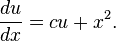
- Inhomogeneous first-order linear constant coefficient ordinary differential equation:
- Homogeneous second-order linear ordinary differential equation:

- Homogeneous second-order linear constant coefficient ordinary differential equation describing the harmonic oscillator:

- First-order nonlinear ordinary differential equation:

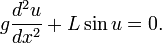
- Second-order nonlinear ordinary differential equation describing the motion of a pendulum of length L:
- Homogeneous first-order linear partial differential equation:

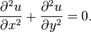
- Homogeneous second-order linear constant coefficient partial differential equation of elliptic type, the Laplace equation:
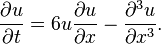
- Third-order nonlinear partial differential equation, the Korteweg–de Vries equation:
Senin, 24 Januari 2011
Linear Programming
Dalam matematika, pemrograman linear ialah teknik optimisasi yang melibatkan variabel-variabel linear. Dalam model pemrograman linear dikenal dua macam fungsi, yaitu fungsi objektif (objective function) dan fungsi kendala (constraint function) yang linear.
Pemrograman linear dapat direpresentasikan dalam notasi matematis sebagai berikut:
Pemrograman linear dapat diterapkan pada berbagai bidang studi. Metode ini paling banyak digunakan dalam bisnis dan ekonomi, namun juga dapat dimanfaatkan dalam sejumlah perhitungan ilmu teknik. Misalnya, dalam ekonomi, fungsi tujuan dapat berkaitan dengan pengaturan secara optimal sumber-sumber daya untuk memperoleh keuntungan maksimal atau biaya minimal, sedangkan fungsi batasan menggambarkan batasan-batasan kapasitas yang tersedia yang dialokasikan secara optimal ke berbagai kegiatan. Industri yang memanfaatkan pemrograman linear di antaranya ialah industri transportasi, energi, telekomunikasi, dan manufaktur. Pemrograman linear juga terbukti berguna dalam membuat model berbagai jenis masalah dalam perencanaan, perancangan rute, penjadwalan, pemberian tugas, dan desain.
Pemrograman linear dapat direpresentasikan dalam notasi matematis sebagai berikut:
- Maksimalkan

- dengan syarat

- dan

Pemrograman linear dapat diterapkan pada berbagai bidang studi. Metode ini paling banyak digunakan dalam bisnis dan ekonomi, namun juga dapat dimanfaatkan dalam sejumlah perhitungan ilmu teknik. Misalnya, dalam ekonomi, fungsi tujuan dapat berkaitan dengan pengaturan secara optimal sumber-sumber daya untuk memperoleh keuntungan maksimal atau biaya minimal, sedangkan fungsi batasan menggambarkan batasan-batasan kapasitas yang tersedia yang dialokasikan secara optimal ke berbagai kegiatan. Industri yang memanfaatkan pemrograman linear di antaranya ialah industri transportasi, energi, telekomunikasi, dan manufaktur. Pemrograman linear juga terbukti berguna dalam membuat model berbagai jenis masalah dalam perencanaan, perancangan rute, penjadwalan, pemberian tugas, dan desain.
Langganan:
Postingan (Atom)